In this blog, I will be comparing a SVM image classifier with a more modern CNN model. I’ll be using the wild-animals-images dataset throughout the blog.

• Old School Approach with SVM
  • Kernel Trick
  • Learning
  • SVM with scikit-learn
    • Loading the Image Data
    • Creating SVM
    • Best Hyperparameters
    • Fitting the remaining data
    • Metrics for best SVM
    • Evaluation with ROC Curve
• Modern Approach with ResNet
  • Loading Data
  • ConvBlock
  • Shortcut connections with Residual Block
  • Putting it all together
  • Training Loop
  • Testing the impact of normalization
  • Evaluation
• Closing Thoughts
• References

Old School Approach with SVM

Support Vector Machine (SVM) is one of the old school methods used for image classification problems. It essentially plots the input features in a n-dimensional space for two classes and attempts to separate the feature data by finding the hyperplane that best isolates the differences in the data.

Kernel Trick

Not all data classes are linearly separable, which is why we typically transform the data into higher dimensional space in such a way so that it becomes linearly separable. We can use a Non-linear Mapping using a kernel to transform the data.

Ex:

Linear Decision Boundary:

\[\vec{w} \cdot \vec{x} + b = 0\]

Non-linear Decision Boundary mapping 2d to 3d space:

\[\vec{w} \cdot \Phi\left(\vec{x}\right) + b = 0 \quad\quad \Phi: \rm I\!R^2 \rightarrow \rm I\!R^3\]

Scikit-learn kernel functions

linear: \(\langle x, x'\rangle\)

polynomial: \(\left(\gamma\langle x, x'\rangle + r\right)^d\) where d specifies the order of the polynomial and r is the coefficient.

rbf: \(\exp\left(-\gamma\| x - x'\|^2\right)\)

sigmoid: \(\tanh\left(\gamma\langle x, x'\rangle + r\right)\)

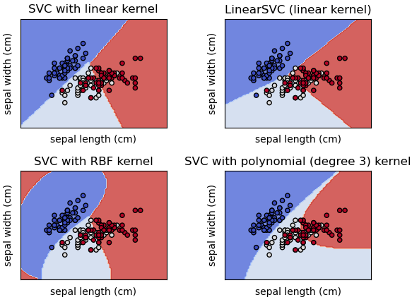
Figure from scikit-learn

Learning

The best hyperplane (decision boundary) is the one that represents the largest margin between the two classes. Sample data points closest to the hyperplane are called the support vectors and are the data points that are chosen for determining the hyperplane. SVM attempts to find the hyperplane with the maximum distance between the support vectors (maximizing the margin).

If you would like to understand more about the learning problem for SVM, I suggest looking at [1] Andrew Nguyen’s notes on SVM.

SVM with scikit-learn

Notebook for the following code

from pathlib import Path
import matplotlib.pyplot as plt
import numpy as np
from sklearn import svm, metrics, datasets
from sklearn.model_selection import GridSearchCV, train_test_split
from skimage.io import imread
import skimage.transform as T

sizes = ["224", "300", "512"]

PATH = "/home/will/Documents/datasets/wild_animals"

Loading the Image Data

When using SVM, one thing you really need to consider is the size of the feature input. We don’t want to have an absurdly large feature vector because it would require a crazy amount of time to train. Also, the number of samples from the datset has to be kept relatively small because it can influence the time complexity by a power of 3.

\[\text{Training time complexity: } \quad O(n_{features} \times n_{samples}^3)\]

def load_image_files(data_dir, lim_sample=None):
    image_dir = Path(data_dir)
    folders = [d for d in image_dir.iterdir() if d.is_dir()]

    x, y = [], []
    for class_idx, direc in enumerate(folders):
        for i, file in enumerate(direc.iterdir()):
            if lim_sample and i >= lim_sample:
                break
            img = imread(file)
            img = T.resize(img, (64, 64, 3))
            x.append(img.flatten()) 
            y.append(class_idx)

    x = np.array(x, dtype=list)
    y = np.array(y, dtype=list).astype(int)

    return x, y 

x, y = load_image_files(PATH + "/" + sizes[0])

I resized the images to be 64x64x3 and flattened them to obtain the feature vector. I’m using the values from the image as the feature input. I have seen more advance techniques used to genereate feature values such as Histogram of Gradients (HOG), but I will be using the more simple approach.

x_train, x_test, y_train, y_test = train_test_split(
    x, y, test_size=0.40, random_state=1234
)
first_x = x_train[:int(len(x_train)*0.4)]
first_y = y_train[:int(len(y_train)*0.4)]
second_x = x_train[int(len(x_train)*0.4):]
second_y = y_train[int(len(y_train)*0.4):] 

In the above code snippet, I did (60/40) split to get a train and test set. For the training data, I did an additional split. The first splits are for seeing which hyperparameters work the best and the second is used to continue training on the rest of the samples with the best SVM. Recall that adding more samples during training will significantly impact training time.

Creating SVM

Scikit-learn offers GridSearchCV which is a useful tool for testing out different hyperparameters in one go. Here you can see that I take advantage of that and test out different gamma, kernel, and C values on the SVM. Parameter C trades off miss-classification against generalizing the decision boundary. The higher the value, the more that it aims to classify the training data correctly. Gamma influences the amount a training sample has, so a higher value would mean that other samples will have to be closer in order to be affected.

hyperparams = [
  {
      'C': [1, 10, 100, 1000],
      'kernel': ['linear']
  },
  {
      'C': [1, 10, 100, 1000],
      'gamma': [1, 0.1, 0.01, 0.001, 0.0001],
      'kernel': ['poly']
  },
  {
      'C': [1, 10, 100, 1000],
      'gamma': [1, 0.1, 0.01, 0.001, 0.0001],
      'kernel': ['sigmoid']
  },
  {
      'C': [1, 10, 100, 1000],
      'gamma': [1, 0.1, 0.01, 0.001, 0.0001],
      'kernel': ['rbf']
  },
]

svc = svm.SVC(probability=True)
grid = GridSearchCV(svc, hyperparams)
grid.fit(first_x, first_y)

Best Hyperparameters

Now we can figure out which parameters performed the best.

print(grid.best_estimator_)
print(grid.best_params_)

Output

SVC(C=10, gamma=0.001, probability=True)
{'C': 10, 'gamma': 0.001, 'kernel': 'rbf'}

Looks like an SVM with C=10, gamma=0.001, and radial basis function kernel performed the best on the dataset.

Fitting the remaining data

from sklearn.metrics import roc_curve, auc, accuracy_score

best_svc = grid.best_estimator_
best_svc.fit(second_x, second_y)

Metrics for best SVM

Using the best SVM, we evaluate the performance of the model. I’ll be using the predicted probabilites of the test data with the actual values to obtain the values needed to create an AUC for the ROC curve.

probs = best_svc.predict_proba(x_test)
y_prob = probs[:, 1]

fpr, tpr, thresholds = roc_curve(y_test, y_prob, pos_label=1)
roc_auc = round(auc(fpr, tpr), 3)

Evaluation with ROC Curve

An ROC curve (receive operating characteristic curve) graphs the performance of a classifier model at all classification thresholds using the True Positive Rate and False Positive Rate.

\[\text{TP rate = }\frac{TP}{TP + FN} \quad\quad\quad \text{FP rate = } \frac{FP}{FP + TN}\]

plt.figure(figsize=(15, 8))
plt.title("ROC curve")
roc_plot = plt.plot(fpr, tpr, label=f"AUC = {roc_auc}")

plt.legend(loc=0)
plt.plot([0,1], [0,1], ls="--")
plt.ylabel("TP Rate")
plt.xlabel("FP Rate")

The ROC represents the degrees of separability, in other words, its a measure for how well the model distinguishes the classes. The AUC represents how often the model predicts the class as correctly right or wrong. This metric will give us more insight into how the model distinguishes the classes. I chose this because with SVM, this would be a better metric because we’re comparing pixel values as opposed to features in the image.

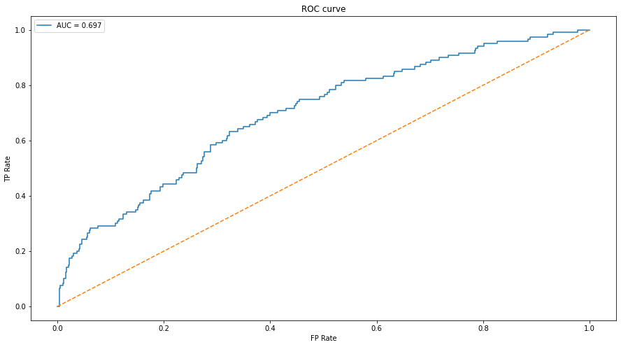
Note that an AUC value < 0.5 would mean that the model is not distinguishing or performing worse than chance. I expected to see an AUC around 0.7-0.8 because of how I defined the feature vector for the model. Also, six classes makes it more difficult to build a solid classifier with SVM just because of the nature of how SVM handles multi-class classification.

Modern Approach with ResNet

[2] Deep Residual Learning for Image Recognition

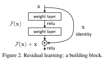
ResNet is a Type of CNN that uses a residual learning framework to facilitate the training on substantially deeper networks. It hypothesizes that it is easier to optimize a residual mapping as opposed to the unreferenced mapping of the stacked layers.

Notebook for the following code

Loading Data

import torch
import torch.nn as nn
import torchvision.datasets as datasets
import torchvision.transforms as T
from torch.utils.data import WeightedRandomSampler, DataLoader
import torch.optim as optim
import matplotlib.pyplot as plt
import numpy as np
import os

sizes = ["224", "300", "512"]

device = "cuda" if torch.cuda.is_available() else "cpu"
classes = ["cheetah", "fox", "hyena", "lion", "tiger", "wolf"]

PATH = "~/Documents/datasets/wild_animals"

I splitted the data (60/40) for train set and test set.

def load_data(path, size, norms):
    data_dir = path + "/" + size
    transform = T.Compose(
        [
            T.Resize((int(size), int(size))),
            T.ToTensor(),
        ]
    )
    dataset = datasets.ImageFolder(root=data_dir, transform=transform)
    
    temp = []
    for (img_t, class_idx) in dataset:
        temp.append((norms[class_idx](img_t), class_idx))
    train_size = int(0.6 * len(dataset))
    test_size = len(dataset) - train_size

    dataset = temp

    train_data, test_data = torch.utils.data.random_split(
        dataset, [train_size, test_size]
    )

    return train_data, test_data

ConvBlock

In the paper, it follows every convolution by a batch norm so I made it its own module.

class ConvBlock(nn.Module):
    def __init__(self, in_channels, out_channels, k_size, stride, pad):
        super(ConvBlock, self).__init__()
        self.conv = nn.Conv2d(in_channels, out_channels, k_size, stride, pad)
        self.bn = nn.BatchNorm2d(out_channels)

    def forward(self, x):
        x = self.conv(x)
        x = self.bn(x)

        return x

Shortcut connections with Residual Block

The residual block uses the identity mapping, meaning the outputs from the shorcut are added to the outputs of the stacked layer. Downsampling is performed on the identity to get the output of the shortcut and then it is added to the output of the other layers.

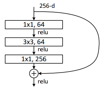
class ResBlock(nn.Module):
    def __init__(self, in_channels, out_channels, down_sample, stride):
        super(ResBlock, self).__init__()
        self.layers = nn.Sequential(
            ConvBlock(in_channels, out_channels, 1, 1, 0),
            ConvBlock(out_channels, out_channels, 3, stride, 1),
            ConvBlock(out_channels, out_channels * 4, 1, 1, 0),
        )
        self.relu = nn.ReLU()
        self.down_sample = down_sample

    def forward(self, x):
        identity = x.clone()
        x = self.layers(x)
        if self.down_sample:
            identity = self.down_sample(identity)
        x += identity
        x = self.relu(x)

        return x

Putting it all together

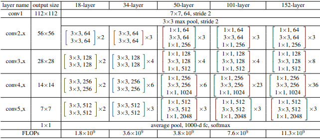
Following the table from above, I constructed the architecture for the ResNet152 the paper claimed performed the best.

class ResNet152(nn.Module):
    def __init__(self, n_classes, depth):
        super(ResNet152, self).__init__()
        self.in_channels = 64
        self.out_channels = 64

        self.conv1 = ConvBlock(depth, self.out_channels, 7, 2, 3)
        self.relu = nn.ReLU()
        self.max_pool = nn.MaxPool2d(3, 2, 1)

        self.conv2_x = self._gen_layer(3, self.out_channels, 1)
        self.out_channels *= 2
        self.conv3_x = self._gen_layer(8, self.out_channels, 2)
        self.out_channels *= 2
        self.conv4_x = self._gen_layer(36, self.out_channels, 2)
        self.out_channels *= 2
        self.conv5_x = self._gen_layer(3, self.out_channels, 2)
        self.avg_pool = nn.AdaptiveAvgPool2d((1, 1))

        self.layers = nn.Sequential(
            self.conv1,
            self.relu,
            self.max_pool,
            self.conv2_x,
            self.conv3_x,
            self.conv4_x,
            self.conv5_x,
            self.avg_pool
        )
        self.fcl = nn.Linear(2048, n_classes)

    def _gen_layer(self, n_res_blocks, out_channels, stride):
        layers = []
        down_sample = ConvBlock(
            self.in_channels, out_channels * 4, 1, stride, 0)

        layers.append(
            ResBlock(self.in_channels, out_channels, down_sample, stride)
        )
        self.in_channels = out_channels * 4

        for _ in range(n_res_blocks - 1):
            layers.append(ResBlock(self.in_channels, out_channels, None, 1))

        return nn.Sequential(*layers)

    def forward(self, x):
        x = self.layers(x)
        x = x.flatten(1)
        x = self.fcl(x)

        return x

Notice that I’m expanding the down_sample ConvBlock by 4 at each residual block and expanding each residual block by 2.

Training Loop

def eval(model, data):
    with torch.no_grad():
        correct = 0

        for (img, label) in data:
            img_input = img.to(device).unsqueeze(0)
            pred = model(img_input)
            _, pred = torch.max(pred.squeeze(), 0)
            pred = pred.to("cpu")
            correct += pred.item() == label
        return correct, round((correct / len(data) * 100), 3)

def train(model, optimizer, train_data, val_data, batch, epochs, lr):
    loader = DataLoader(
        train_data,
        batch_size=batch,
        shuffle=True,
        num_workers=2,
    )
    criterion = nn.CrossEntropyLoss()

    epoch_data = []
    for epoch in range(epochs):
        running_loss, running_acc = 0., 0.
        for i, (imgs, labels) in enumerate(loader):
            inputs, labels = imgs.to(device), labels.to(device)
            optimizer.zero_grad()

            outputs = model(inputs)
            loss = criterion(outputs, labels)
            loss.backward()
            optimizer.step()

            running_loss += loss.item()
            _, pred = torch.max(outputs, dim=1)
            running_acc += torch.sum(pred == labels).item()

        model.eval()
        _, val_acc = eval(model, val_data)
        model.train()

        running_acc = round(running_acc / len(train_data) * 100, 3)
        running_loss /= len(loader)
        print(f'epoch: {epoch + 1} loss: {running_loss:.6f}')
        epoch_data.append(
            (epoch, float(f"{(running_loss):.6f}"), running_acc, val_acc)
        )
    
    return epoch_data

Testing the impact of normalization

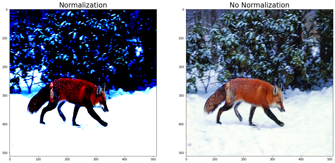
Normalizing the image before training creates more stability for the optimizer during training. Theoretically, we should arrive at a better accuracy with the normalized dataset given the same number of epochs. I’ll be experimenting with both to see which one performs the best.

def norm_transforms(path, size):
    data_dir = path + "/" + size
    transforms = T.Compose(
        [T.Resize((int(size), int(size))), T.ToTensor()]
    )
    dataset = datasets.ImageFolder(root=data_dir, transform=transforms)

    imgs = {}
    for img_t, class_idx in dataset:
        if class_idx in imgs:
            imgs[class_idx].append(img_t)
        else:
            imgs[class_idx] = [img_t]

    norms, unnorms = {}, {}
    for i in range(len(imgs)):
        imgs[i] = torch.stack(imgs[i], dim=3)
        mean = np.array([m for m in imgs[i].view(3, -1).mean(dim=1)])
        std = np.array([s for s in imgs[i].view(3, -1).std(dim=1)])

        norms[i] = T.Normalize(
            mean = mean,
            std = std
        )
        unnorms[i] = T.Normalize(
            mean = -(mean/std),
            std = (1 / std)
        )
    
    return norms, unnorms

Notice that I normalized the dataset based on the values for each class rather than the values of the dataset as a whole.

Showing the effects of normalization on an image.

test_img, class_idx = train_data[np.random.randint(0, len(train_data))]
imgs = [
    test_img.permute(1, 2, 0), unnorms[class_idx](test_img).permute(1, 2, 0)
]

fig, axs = plt.subplots(1, 2, figsize=(20, 12))
axs[0].set_title("Normalization", fontsize=24)
axs[1].set_title("No Normalization", fontsize=24)
axs[0].imshow(imgs[0])
axs[1].imshow(imgs[1])

Running the model on the dataset with and without normalization.

import gc

def run(norm):
    lr = 0.01
    batch_size = 32
    num_epochs = 100
    runs = []
    size = sizes[0]

    if norm:
        train_data, val_data = load_data(PATH, size, norms)
    else:
        train_data, val_data = load_data(PATH, size, unnorms)

    model = ResNet152(len(classes), 3).to(device)
    opt = optim.SGD(
        model.parameters(), lr=lr, weight_decay=0.0001, momentum=0.9)
    epoch_data = train(
        model,
        opt,
        train_data,
        val_data,
        batch_size,
        num_epochs,
        lr
    )
    runs.append(epoch_data)
    del opt
    del model
    gc.collect()
    torch.cuda.empty_cache()

    return runs

In the paper, SGD with weight_decay=0.0001 and momentum=0.9 is used for the optimizer. I used Binary Cross Entropy loss for training as that is the standard criterion for image classification with CNNs.

Evaluation

epoch_data = []
epoch_data += run(False)
epoch_data += run(True)

def plot_data(norm):
    train_info = [*zip(*epoch_data[int(norm)])]
    train_acc = np.array(train_info[2]) / 100
    test_acc = np.array(train_info[-1]) / 100

    fig, axs = plt.subplots(1, 2, figsize=(24, 8))
    axs[0].set_title("ResNet152 Loss", fontsize=20)
    axs[1].set_title("ResNet152 Accuracy", fontsize=20)

    axs[0].plot(train_info[0], train_info[1], color="red")
    axs[1].plot(train_info[0], train_acc, color="orange")
    axs[1].plot(train_info[0], test_acc, color="blue")

    axs[0].set_xlabel("Epoch", fontsize=16)
    axs[0].set_ylabel("Loss", fontsize=16)
    axs[1].set_xlabel("Epoch", fontsize=16)
    axs[1].set_ylabel("Accuracy", fontsize=16)

    print(f"ResNet train accuracy: {train_acc[-1]:.3f}")
    print(f"ResNet test accuracy: {test_acc[-1]:.3f}")

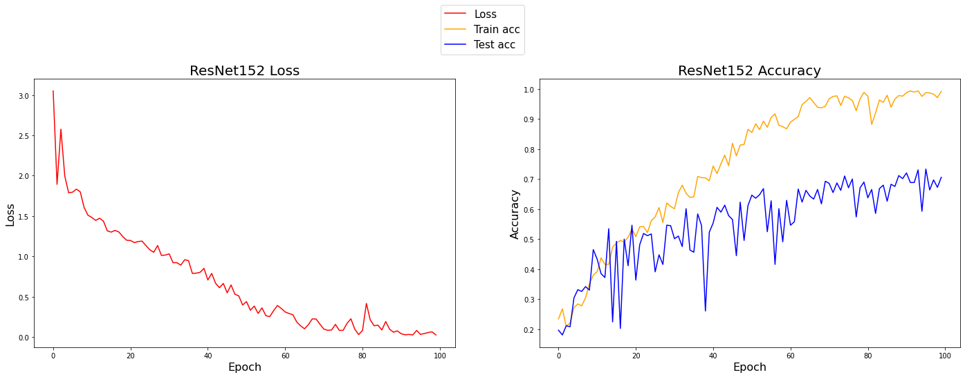
plot_data(norm=False)

No Normalization

Output

ResNet train accuracy: 0.992
ResNet test accuracy: 0.706

plot_data(norm=True)

With Normalization

Output

ResNet train accuracy: 0.932
ResNet test accuracy: 0.728

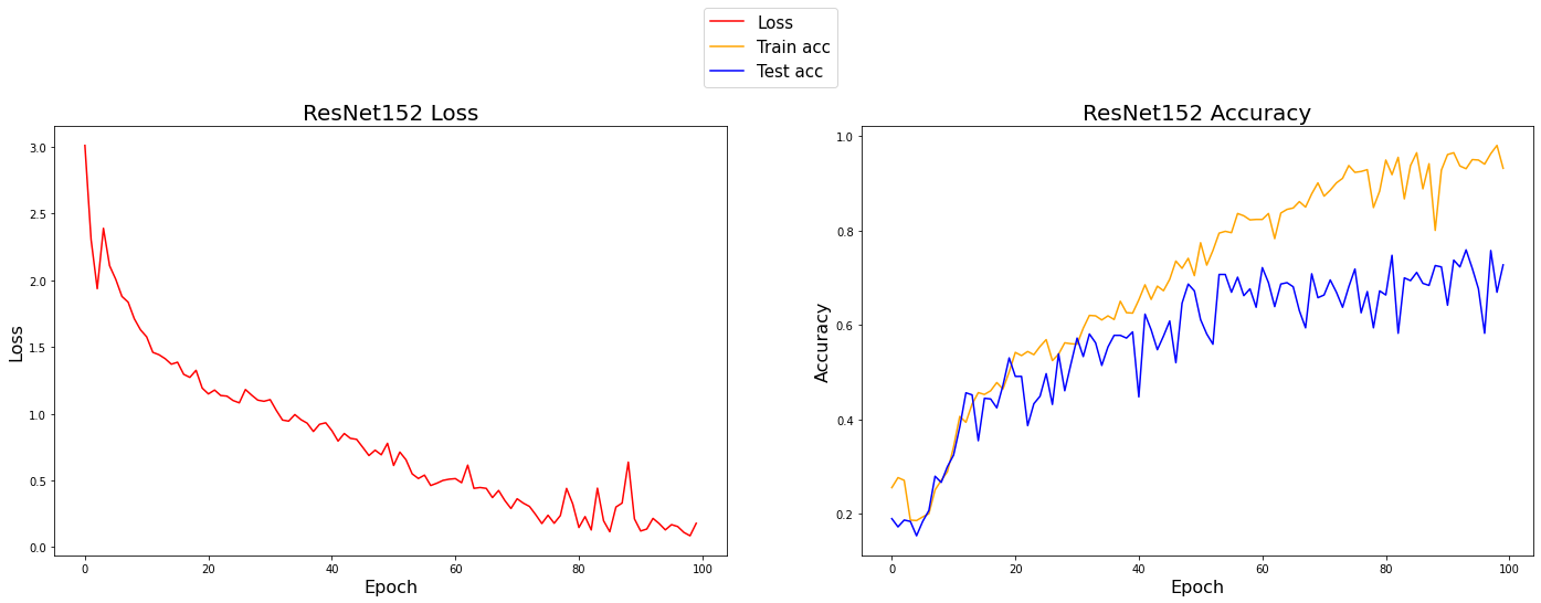
Looking at the test accuracy curves, you may notice that the dips on the data without normalization are much greater than the dips with normalization. This shows that the normalization technique does provide some stability, and it also looks like the final accuracy was slightly better by roughly 2%. Contrasting the train and test accuracies, it appears that normalization generalizes better.

Closing Thoughts

There are a few things that can be compared when looking at the different types of models used for the image classification.

One thing I did not mention was the amount of time spent for training each. With the SVM, it took my machine roughly 40 minutes to train the SVM with the different hyperparameters, which made it easier to adjust and play around with. With ResNet, It took me nearly two hours to train both models, so I couldn’t really change much with the model as it would have taken far too long. Also, I’m sure I could have improved both of the models by a relatively considerable amount if I had used more features for the SVM or iterations for the CNN.

An advantage that the SVM had was that it was easier to set up and toy around with whereas I struggled quite a bit when implementing the ResNet model. The downside is that it doesn’t classify as well as ResNet.

References

[1] Nguyen, Andrew. Part V Support Vector Machines - Stanford Engineering Everywhere. https://see.stanford.edu/materials/aimlcs229/cs229-notes3.pdf

[2] He, Kaiming, et al. “Deep Residual Learning for Image Recognition.” ArXiv.org, 10 Dec. 2015, https://arxiv.org/abs/1512.03385