Image Classification with ConvNets
Convolutional neural networks have played a critical role in solving image classification problems and is typically the first type of machine learning model considered for building image classifiers.
- What is convolution?
- Convolutional Neural Networks with PyTorch
- VGGNet implementation
- GoogLeNet implementation
What is convolution?
It’s important to understand the key component that drives convolutional neural networks and why it performs so well in image classification. The convolutional layer is the defining feature of this type of neural network. This layer is responsible for learning features that belong to a class. It accomplishes this by applying a filter (kernel) on the receptive fields (local regions) of the input image, resulting in a feature map. Mathematically, this operation is done by applying the element-wise product between all of the receptive fields and the kernel, then summing every element in each receptive field, and finally mapping the summed values to the feature map.
For example:
\[A = \begin{bmatrix} 0 & 0.5 & 0 & 0 \\ 0 & 0.5 & 0 & 0 \\ 0 & 0.5 & 0.5 & 0.5 \\ 0 & 0.5 & 0 & 0 \end{bmatrix} B = \begin{bmatrix} 0 & 1 \\ 0 & 1 \end{bmatrix}\]Let A represent a grayscale image and B be a 2x2 kernel used for detecting vertical edges in A. If we perform convolution with a stride of 2 and no padding, then our receptive fields would be the four 2x2 corners of A shown below.
\[S = \left[ \begin{array}{c|c} S_{11} & S_{12} \\ \hline S_{21} & S_{22} \end{array} \right] = \left[\begin{array}{c|c} \begin{bmatrix} 0 & 1 \\ 0 & 1 \end{bmatrix} & \begin{bmatrix} 0 & 0 \\ 0 & 0 \end{bmatrix} \\ \hline \begin{bmatrix} 0 & 1 \\ 0 & 1 \end{bmatrix} & \begin{bmatrix} 1 & 1 \\ 0 & 0 \end{bmatrix} \end{array}\right]\]Apply the kernel to each receptive field and sum the elements to the resulting feature map.
The size of the feature map \(n_{out}\) depends on the size of the input \(n_{in}\), stride \(s\), padding \(p\), and kernel \(k\). In the example, \(n_{in}\) = 4 reduced to \(n_{out}\) = 2, but typically we want \(n_{in}\) = \(n_{out}\) as you’ll see later.
\[n_{out}=\dfrac{n_{in} + 2p - k}{s} + 1\]This is a very basic example, but it highlights the intuition behind convolution. We’re essentially trying to exaggerate a feature we’re looking for in an image. In this case, the vertical edge became more pronounced in the output image.
In computer vision, this process is used for image filtering and there are a variety of filters used for specific purposes such as edge detection and noise removal. When we’re dealing with image classification, it would be difficult to come up with the values of a filter for picking out parts of a body such as hair. Furthermore, hair can come in many different shapes and colors. This is where convolution in neural networks excel at. We can have the neural network come up with the best values (weights) for a filter automatically with a convolutional layer. Additionally, we can apply as many filters as we want at each layer.
More on ConvNets
Another key component in convolutional neural networks is the pooling layer. Generally, the location of a feature is only significant when accounting for neighboring features. For example, the defining features of a face are eyes, nose, and mouth. In an image, these features need to be near each other to define a face. However, the location of the face in the image is insignifcant. Max pooling is a common technique that can be applied periodically throughout the network to downsample (also known as subsampling), reducing the number of parameters in the network while being locally shift invariant. In max pooling, the largest value that lies within a filter is kept.
For example: with kernel size and shift of 2
\[\begin{bmatrix} 2 & 0 & 0 & 3 \\ \underline{\textbf{3}} & 1 & \underline{\textbf{5}} & 1 \\ 2 & 0 & 0 & \underline{\textbf{2}} \\ \underline{\textbf{3}} & 1 & 1 & 1 \\ \end{bmatrix} \xrightarrow{\text{maxpool}} \begin{bmatrix} 3 & 5 \\ 3 & 2 \end{bmatrix}\]These two components are essential for any convolutional network, so understanding how each work will make understanding ConvNets simple.
Convolutional Neural Networks with PyTorch
I’ll be demonstrating my attempt at CNNs with Caltech101 | Airplanes, Motorbikes & Schooners
For the sake of brevity, I will only explain the code segments that are relavent towards the topic and will not re-explain code that has already been shown. The notebook is available Here
import torch
import torch.nn as nn
import torchvision.datasets as datasets
import torchvision.transforms as transforms
from torch.utils.data import WeightedRandomSampler, DataLoader
import torch.optim as optim
import matplotlib.pyplot as plt
import numpy as np
import os

NUM_CLASSES = 3
CHANNELS_D = 3
IMG_SIZE = 256
DATA_DIR = "/home/will/Documents/datasets/archive/caltech101_classification/"

device = "cuda" if torch.cuda.is_available() else "cpu"
classes = ["Motorcycle", "Airplane", "Schooner"]
Data
Normalizing the image data reduces the chance of vanishing and exploding gradients for the optimizer during training. To do this, calculate the mean \(\mu\) and standard deviation \(\sigma\) of each channel for every image in the dataset, then subtract each value by its respective mean and divide by its standard deviation.
\[Z = \dfrac{x - \mu}{\sigma}\]PyTorch does the Normalization part for us
# for simplicity, just normalize whole dataset instead of each class label
def norm_transforms():
transform = transforms.Compose(
[transforms.Resize((IMG_SIZE, IMG_SIZE)), transforms.ToTensor()]
)
dataset = datasets.ImageFolder(root=DATA_DIR, transform=transform)
# concat image data (CxWxH) in tensor, discard labels
imgs = torch.stack([img_t for img_t, _ in dataset], dim=3)
# flatten the three channels of all images and take the mean
mean = np.array([m for m in imgs.view(3, -1).mean(dim=1)])
std = np.array([s for s in imgs.view(3, -1).std(dim=1)])
norm = transforms.Normalize(
mean = mean,
std = std
)
unnorm = transforms.Normalize(
mean = -(mean/std),
std = (1 / std)
)
return norm, unnorm
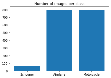
norm, unnorm = norm_transforms()Since the number of images for schooner class is dramatically smaller than the other two classes in the dataset, I computed some weights to apply for the loss criterion during training by taking the difference of each portion by 1.
import pandas as pd

class_weights = []
total_len = 0
for _, _, files in os.walk(DATA_DIR):
    if len(files) > 0:
        class_weights.append(len(files))
    total_len += len(files)
plt.bar(classes[::-1], class_weights)
plt.title("Number of images per class")
plt.show()

class_weights = np.round((1 - np.array(class_weights) / total_len), 3)
class_weights = class_weights.tolist()

print("Class_weights")
df = pd.Series(classes[::-1], class_weights)
class_weights = torch.tensor(class_weights)

df
Output
Class_weights
0.962      Schooner
0.518      Airplane
0.520    Motorcycle
dtype: object
The next step is to apply the transformations (Resizing each image to the same size and normalizing) and split the dataset. I originally planned on doing 60/20/20 split for a train, validation, and test set. However, I found that a 20/20 split would be too small and since I was testing a variety of different networks in one go, I wouldn’t need to do much tuning. Ultimately, I decided on a 60/40 split and commented out the former.
def load_data():
    transform = transforms.Compose(
        [
            transforms.Resize((IMG_SIZE, IMG_SIZE)),
            transforms.ToTensor(),
            norm,
        ]
    )
    dataset = datasets.ImageFolder(root=DATA_DIR, transform=transform)

    train_size = int(0.6 * len(dataset))
    test_size = len(dataset) - train_size

    train_data, test_data = torch.utils.data.random_split(
        dataset, [train_size, test_size]
    )

    return train_data, test_data
    # train_data, test_val_data = torch.utils.data.random_split(
    #     dataset, [train_size, test_val_size]
    # )

    # val_size = int(0.5 * len(test_val_data))
    # test_size = len(test_val_data) - val_size
    # val_data, test_data = torch.utils.data.random_split(
    #     test_val_data, [val_size, test_size]
    # )
    # return train_data, val_data, test_data

# train_data, val_data, test_data = load_data()
train_data, val_data = load_data()
My attempt at CNNs
class CNN(nn.Module):
    def __init__(self, num_layers, expansion):
        super().__init__()
        self.fcl, self.net = self._gen_layers(num_layers, expansion)
        self.classifier = self._classifier()

    def _gen_layers(self, num_layers, expansion):
        layers = []
        in_channels = CHANNELS_D

        for i in range(num_layers):
            out_channels = expansion(in_channels)
            layers += [
                nn.Conv2d(in_channels, out_channels, kernel_size=5, padding=2)
            ]
            layers += [nn.ReLU(), nn.BatchNorm2d(out_channels)]
            layers += [nn.MaxPool2d(2, 2)]
            in_channels = out_channels
        fcl = ((IMG_SIZE // (2 ** num_layers)) ** 2) * in_channels

        return fcl, nn.Sequential(*layers)

    def _classifier(self):
        layers = [
            nn.Flatten(1),
            nn.Linear(self.fcl, 256),
            nn.ReLU(),
            nn.Linear(256, NUM_CLASSES)
        ]

        return nn.Sequential(*layers)

    def forward(self, x):
        return self.classifier(self.net(x))
The way this network is structured can be explained by gen_layers. It takes in num_layers(the number of convolutional layers), and expansion which is a lambda expression used for expanding the number of feature maps from each conv layer. Each conv layer is followed by ReLU activation function, BatchNorm, and MaxPool. The sequence is stored in self.net on construction.
classifier contains the fully connected layers that result in the model’s prediction and is generated on construction.
The forward pass throws the input through the sequence of conv layers in self.net, then passes the output from the self.net to the sequence of fully connected layers from classifier to get the prediction.
Notice
fcl = ((IMG_SIZE // (2 ** num_layers)) ** 2) * in_channelsThis expression represents the number of neurons in each feature map multiplied by the number of feature maps at the end of gen_layers. Recall that maintaining dimensionality of the feature maps \(n_{in}\) = \(n_{out}\) makes computing this value convenient.
Metrics for training
def eval(model, data):
    with torch.no_grad():
        correct = 0

        for (img, label) in data:
            img_input = img.to(device).unsqueeze(0)
            pred = model(img_input)
            _, pred = torch.max(pred.squeeze(), 0)
            pred = pred.to("cpu")
            correct += pred.item() == label
        return correct, round((correct / len(data) * 100), 3)

def count_params(model: nn.Module):
    return sum(p.numel() for p in model.parameters() if p.requires_grad)
This function scores the percent accuracy and number of correct classifications.
Training loop
def train(model, train_data, val_data, batch, epochs, lr, class_weights):
    loader = DataLoader(
        train_data,
        batch_size=batch,
        shuffle=True,
        num_workers=2,
    )
    criterion = nn.CrossEntropyLoss(weight=class_weights.to(device))
    optimizer = optim.SGD(model.parameters(), lr=lr)

    epoch_data = []
    for epoch in range(epochs):
        running_loss, running_acc = 0.0, 0.0
        for i, (imgs, labels) in enumerate(loader):
            inputs, labels = imgs.to(device), labels.to(device)
            optimizer.zero_grad()

            outputs = model(inputs)
            loss = criterion(outputs, labels)
            loss.backward()
            optimizer.step()

            running_loss += loss.item()
            _, pred = torch.max(outputs, dim=1)
            running_acc += torch.sum(pred == labels).item()

        model.eval()
        _, val_acc = eval(model, val_data)
        model.train()

        running_acc = round(running_acc / len(train_data) * 100, 3)
        running_loss /= len(loader)
        print(f'epoch: {epoch + 1} loss: {running_loss:.6f}')
        epoch_data.append(
            (epoch, float(f"{(running_loss):.6f}"), running_acc, val_acc)
        )

    return epoch_data
This is the standard training loop for a PyTorch model. Only things noteworthy here are the criterion and optimizer.
Notice
criterion = nn.CrossEntropyLoss(weight=class_weights.to(device))I used the class weights I calculated earlier with the Cross Entropy Loss function. For the optimizer, I used Stochastic Gradient Descent with a learning rate specific to each model.
Test out CNNs
expansions = []
lrs = [1e-4, 2e-3, 35e-4, 0.01]
num_layers = 4
batch_size = 128
num_epochs = 20

# recursive expressions to use for expanding feature map from conv layer
expansions.append(lambda x: x + 13)
expansions.append(lambda x: x*2 if x < 20 else x + (x // 2))
expansions.append(lambda x: x*3 if x < 50 else x + (x // 6))

runs = []
for n in range(num_layers):
    for expr in expansions:
        model = CNN(n + 1, expr).to(device)
        epoch_data = train(
            model,
            train_data,
            val_data,
            batch_size,
            num_epochs,
            lrs[n],
            class_weights
        )
        print("evaluating...")
        model.eval() # set eval for batch norm bc batch size is only 1
        n_params = count_params(model)
        runs.append((n, expr, n_params, epoch_data))
        del model
In the above code segment, I’m evaluating different CNN architectures based on number of convolutional layers and number of feature maps from each layer.
Plotting losses and accuracies
def str_conv_seq(expr, n_lay):
prior = CHANNELS_D
conv_seq = str(prior)
total = 0
for i in range(n_lay + 1):
prior = expr(prior)
total += prior
conv_seq += f"->{str(prior)}"
conv_seq
return conv_seq, total
def plot_losses(runs):
fig, axs = plt.subplots(1, len(expansions), figsize=(28,6),
gridspec_kw={'wspace': 0}, sharey=True)
axs[0].set_ylabel("loss", fontsize=15)
for (n_lay, expr, n_params, epoch_data) in runs:
c = expansions.index(expr)
conv_seq, _ = str_conv_seq(expr, n_lay)
train_info = [*zip(*epoch_data)]
axs[c].set_title(
"Feature Map Expansion: " + conv_seq, fontsize=15
)
if c == len(expansions) - 1:
axs[c].plot(
train_info[0],
train_info[1],
label=f"{n_lay + 1} conv layers"
)
else:
axs[c].plot(train_info[0], train_info[1])
for ax in axs:
ax.set_xlabel("epoch", fontsize=15)
ax.set_xticks(np.arange(0, num_epochs + 1, 5))
lines_labels = [ax.get_legend_handles_labels() for ax in fig.axes]
lines, labels = [sum(l_l, []) for l_l in zip(*lines_labels)]
fig.legend(lines, labels, fontsize=15, loc="upper center")
fig.subplots_adjust(top=0.7)
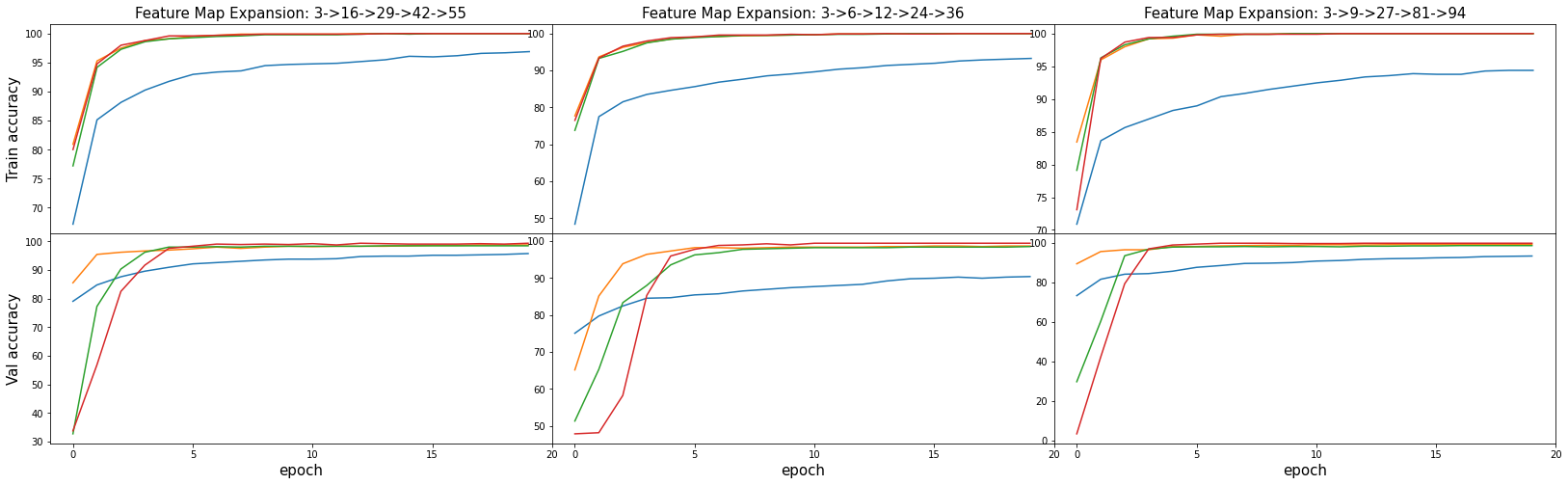
def plot_accuracies(runs):
fig, axs = plt.subplots(2, len(expansions), figsize=(28,8),
gridspec_kw={'hspace': 0, 'wspace': 0})
axs[0, 0].set_ylabel('Train accuracy', fontsize=15)
axs[1, 0].set_ylabel('Val accuracy', fontsize=15)
for (n_lay, expr, n_params, epoch_data) in runs:
c = expansions.index(expr)
conv_seq, _ = str_conv_seq(expr, n_lay)
train_info = [*zip(*epoch_data)]
if c == len(expansions) - 1:
axs[0, c].plot(
train_info[0],
train_info[2],
label=f"{n_lay + 1} conv layers"
)
else:
axs[0, c].plot(train_info[0], train_info[2])
axs[0, c].set_title(
"Feature Map Expansion: " + conv_seq, fontsize=15
)
axs[1, c].plot(train_info[0], train_info[3])
for ax in axs[1, :]:
ax.set_xlabel("epoch", fontsize=15)
ax.set_xticks(np.arange(0, num_epochs + 1, 5))
plot_losses(runs)
plot_accuracies(runs) 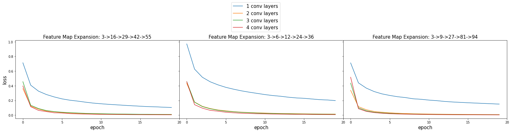
def show_final_acc(runs):
    convs = []
    for (n_lay, expr, _, epoch_data) in runs:
        conv_seq, total = str_conv_seq(expr, n_lay)
        conv_seq += f" FM total: {total}"
        convs.append((f"{epoch_data[-1][-1]}%", conv_seq))
    df = pd.Series(*zip(*convs))
    print("accuracies on validation set")
    return df

show_final_acc(runs)
Output
accuracies on validation set
3->16 FM total: 16                 95.789%
3->6 FM total: 6                   90.376%
3->9 FM total: 9                   93.233%
3->16->29 FM total: 45             98.797%
3->6->12 FM total: 18              98.647%
3->9->27 FM total: 36              99.098%
3->16->29->42 FM total: 87         98.496%
3->6->12->24 FM total: 42          98.496%
3->9->27->81 FM total: 117         98.496%
3->16->29->42->55 FM total: 142    99.398%
3->6->12->24->36 FM total: 78      99.398%
3->9->27->81->94 FM total: 211     99.699%
dtype: object
What I learned
Expanding the number of feature maps at each conv layer doesn’t seem to have any meaningful influence on the performance. It does appear to perform better the deeper the network gets, the last three runs with four conv layers all performed > 99.0%. I was satisfied with the results, with the best conv net having a score of 99.699% correct.
I also tried implementing a few popular ConvNet architectures that interested me for fun.
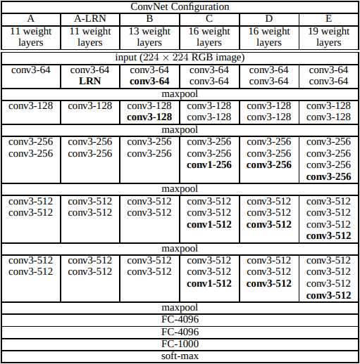
VGGNet implementation
[1] Very Deep Convolutional Networks for Large-Scale Image Recognition
Notes
- Conv layers use 3x3 kernel with the exception of C
- C uses 1x1 kernel at the end of the last three sections
- Padding used on convolutions to maintain dimensionality of input
- Maxpool between each section of conv layers uses 2x2 for kernel and stride
- Maxpool is followed by ReLU
The original VGG didn’t include batchnorm operations in the model, so that is something I included. Another thing to note is the image size they used. They used 224x224, however, my images will remain 256x256. I will not be experimenting with A-LRN, as the paper concluded that it did not improve performance and only increased memory usage and computation time.
I didn’t include softmax on the output because I’m using cross entropy loss (CEL) as my loss function. Generally, the combination of both would introduce vanishing gradient problem because PyTorch incorporates softmax into CEL by default. See torch.nn.CrossEntropyLoss
I had orignally included it to see what my results would look like. The loss struggled to decrease and the model wouldn’t improve.
Model
class VGG(nn.Module):
    def __init__(self, net_config=None):
        super().__init__()
        self.configs = {         # not including A-LRN for convenience
            'A': [1, 1, 2, 2, 2],
            'B': [2, 2, 2, 2, 2],
            'C': [2, 2, 3, 3, 3],
            'D': [2, 2, 3, 3, 3],
            'E': [2, 2, 4, 4, 4]
        }
        if net_config:
            self.fcl, self.net = self._gen_layers(net_config)
            self.classifier = self._classifier()

    def _gen_layers(self, net_config):
        layers = []
        num_layers = self.configs[net_config]
        in_channels, out_channels = CHANNELS_D, 64

        for i, n in enumerate(num_layers):
            for j in range(1, n + 1):
                c_trans = net_config == "C" and j == n and out_channels >= 256
                (kernel, pad) = (1, 0) if c_trans else (3, 1)
                layers.append(nn.Conv2d(
                        in_channels, out_channels, kernel, padding=pad
                    )
                )
                layers.append(nn.BatchNorm2d(out_channels))
                layers.append(nn.ReLU())
                in_channels = out_channels
            layers.append(nn.MaxPool2d(2, 2))
            if out_channels < 512:
                out_channels *= 2
        fcl = ((IMG_SIZE // (2 ** 5)) ** 2) * in_channels

        return fcl, nn.Sequential(*layers)

    def _classifier(self):
        layers = []
        layers += [
            nn.Flatten(1),
            nn.Linear(self.fcl, 4096), nn.ReLU(),
            nn.Linear(4096, 4096), nn.ReLU(),
            nn.Linear(4096, NUM_CLASSES)
        ]

        return nn.Sequential(*layers)

    def forward(self, x):
        return self.classifier(self.net(x))
The model is very basic and structured similarly to how I designed my vanilla CNN architecture. The main distinction being the number of conv layers used. Also, a conv layer will expand the number of feature maps less frequently and only by a factor of 2 starting from 64.
Evaluation
runs_vgg = []
batch_size = 16
num_epochs = 30
lr = 1e-3

for (vgg_arch, layers) in VGG().configs.items():
    model = VGG(vgg_arch).to(device)
    epoch_data = train(
        model,
        train_data,
        val_data,
        batch_size,
        num_epochs,
        lr,
        class_weights
    )
    print("evaluating...")
    model.eval()
    _, accuracy = eval(model, val_data)
    runs_vgg.append((
        "VGG-" + str(np.sum(layers)) + vgg_arch,
        n_params,
        epoch_data
    ))
    del model
def subtitle(fig, grid, title):
row = fig.add_subplot(grid)
row.set_title(f'{title}', fontweight='semibold')
row.set_frame_on(False)
row.axis('off')
def plot_runs(runs):
fig, axs = plt.subplots(len(runs), 2, figsize=(12,18))
grid = plt.GridSpec(len(runs), 2)
for i, (label, accuracy, epoch_data) in enumerate(runs):
train_info = [*zip(*epoch_data)]
axs[i, 0].set(ylabel="loss")
axs[i, 1].set(ylabel="accuracy")
axs[i, 0].plot(train_info[0], train_info[1], label=label)
axs[i, 1].plot(train_info[0], train_info[2], label="train")
axs[i, 1].plot(
train_info[0], train_info[3], linestyle="dashed", label="val"
)
subtitle(fig, grid[i, ::], label)
for ax in axs:
ax[0].set(ylabel="loss")
ax[1].set(ylabel="accuracy")
ax[0].set(xlabel="epoch")
ax[1].set(xlabel="epoch")
lines_labels = [ax.get_legend_handles_labels() for ax in axs[0][1:]]
lines, labels = [sum(l_l, []) for l_l in zip(*lines_labels)]
fig.legend(lines, labels, loc='center right')
plt.show()
plot_runs(runs_vgg)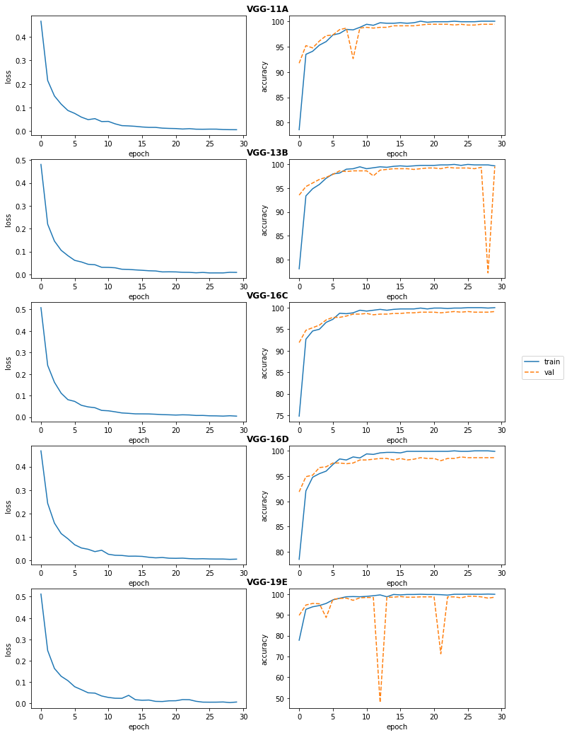
Looking at the accuracy for the validation set, there are massive dips in some of the models. If you look closely, you can correspond these dips to an increase on the loss curve at the same epoch, which would explain the drop in accuracy.
def show_final_acc(runs):
    convs = []
    for (arch, n_params, epoch_data) in runs:
        convs.append((f"{epoch_data[-1][-1]}%", arch))
    df = pd.Series(*zip(*convs))
    print("accuracies on validation set")
    return df

show_final_acc(runs_vgg)
Output
accuracies on validation set
VGG-11A 99.398%
VGG-13B 99.549%
VGG-16C 99.098%
VGG-16D 98.647%
VGG-19E 98.496%
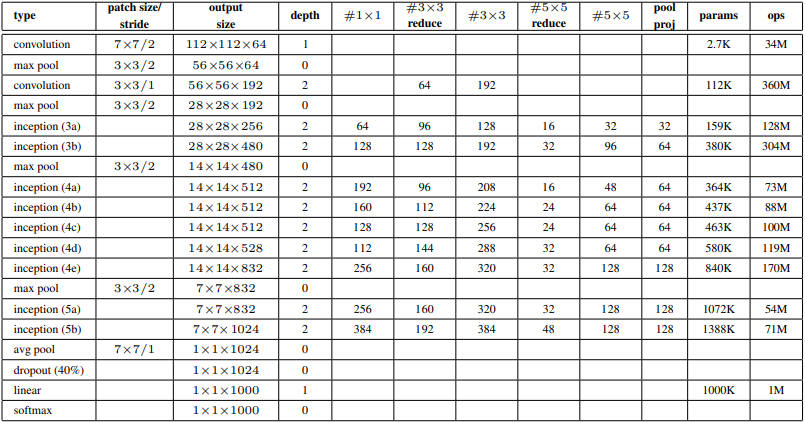
dtype: objectGoogLeNet implementation
[2] Going Deeper with Convolutions
Architecture
The changes I made from the original VGG net architecture can pratically be applied here. Original GoogLeNet didn’t use batchnorms, it used softmax, and trained on 224x224 images.
Same sequences of operations following a convolution as the other networks, but this time I made it into its own class to be applied repeatedly throughout the network.
class Conv(nn.Module):
    def __init__(self, in_channels, out_channels, **kwargs):
        super().__init__()
        self.conv  = nn.Sequential(
            nn.Conv2d(in_channels, out_channels, **kwargs),
            nn.BatchNorm2d(out_channels),
            nn.ReLU()
        )

    def forward(self, x):
        return self.conv(x)
Inception block
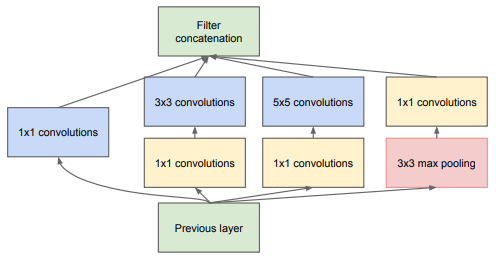
This block is responsible for deciding which kernel sizes contribute the most on a given input in the network. Since using 3x3 and 5x5 filters can be computationally expensive, they apply 1x1 filters before them to reduce the number of input features for those conv layers.
class Inception(nn.Module):
    def __init__(self, in_channels, _1x1, _3x3r, _3x3, _5x5r, _5x5, pool):
        super().__init__()
        self.inc_block = self._gen_branches(
            in_channels, _1x1, _3x3r, _3x3, _5x5r, _5x5, pool
        )

    def _gen_branches(self, in_channels, _1x1, _3x3r, _3x3, _5x5r, _5x5, pool):
        b1 = nn.Sequential(Conv(in_channels, _1x1, kernel_size=1).to(device))
        b2 = nn.Sequential(
            Conv(in_channels, _3x3r, kernel_size=1).to(device),
            Conv(_3x3r, _3x3, kernel_size=3, padding=1).to(device)
        )
        b3 = nn.Sequential(
            Conv(in_channels, _5x5r, kernel_size=1).to(device),
            Conv(_5x5r, _5x5, kernel_size=5, padding=2).to(device)
        )
        b4 = nn.Sequential(
            nn.MaxPool2d(3, 1, 1),
            Conv(in_channels, pool, kernel_size=1).to(device)
        )

        return [b1, b2, b3, b4]

    def forward(self, x):
        return torch.cat([b(x) for b in self.inc_block], dim=1)
Model
I constructed the layers for the network using the same values in the same order from the table above.
class GoogLeNet(nn.Module):
    def __init__(self):
        super().__init__()
        self.layers = self._gen_layers()
        self.classifier = self._classifier()

    def _gen_layers(self):
        layers = [
            Conv(3, 64, kernel_size=7, stride=2, padding=3),
            nn.MaxPool2d(3, 2, 1),
            Conv(64, 192, kernel_size=3, stride=1, padding=1),
            nn.MaxPool2d(3, 2, 1),
            Inception(192, 64, 96, 128, 16, 32, 32),
            Inception(256, 128, 128, 192, 32, 96, 64),
            nn.MaxPool2d(3, 2, 1),
            Inception(480, 192, 96, 208, 16, 48, 64),
            Inception(512, 160, 112, 224, 24, 64, 64),
            Inception(512, 128, 128, 256, 24, 64, 64),
            Inception(512, 112, 144, 288, 32, 64, 64),
            Inception(528, 256, 160, 320, 32, 128, 128),
            nn.MaxPool2d(3, 2, 1),
            Inception(832, 256, 160, 320, 32, 128, 128),
            Inception(832, 384, 192, 384, 48, 128, 128),
        ]

        return nn.Sequential(*layers)

    def _classifier(self):
        feature_map_dim = IMG_SIZE // (2 ** 5)
        layers = [
            nn.AvgPool2d(feature_map_dim, 1),
            nn.Flatten(1),
            nn.Dropout(0.4),
            nn.Linear(1024, NUM_CLASSES)
        ]

        return nn.Sequential(*layers)

    def forward(self, x):
        x = self.layers(x)
        x = self.classifier(x)

        return x
Evaluation
runs_google = []
batch_size = 64
num_epochs = 100
lr = 1e-3

model = GoogLeNet().to(device)
epoch_data = train(
        model,
        train_data,
        val_data,
        batch_size,
        num_epochs,
        lr,
        class_weights
    )
print("evaluating...")
n_params = count_params(model)
runs_google.append(("GoogLeNet", n_params, epoch_data))
del model
train_info = [*zip(*runs_google[0][2])]
acc = np.array(train_info[2]) / 100
plt.figure(figsize=(12,6))
plt.title("GoogLeNet", fontsize=15)
plt.plot(train_info[0], train_info[1], label="GoogLeNet Loss")
plt.plot(train_info[0], acc, label="GoogLeNet Accuracy", linestyle="dashed")
plt.legend()
print(f"GoogLeNet accuracy: {train_info[0][-1]:.3f}")Output
GoogLeNet accuracy: 99.000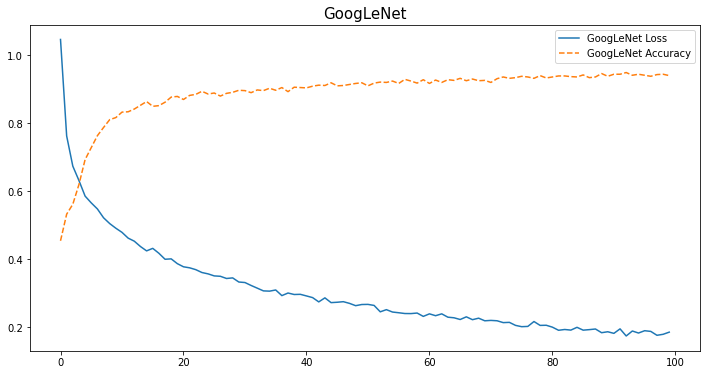
References
[1] Simonyan, Karen, and Andrew Zisserman. “Very Deep Convolutional Networks for Large-Scale Image Recognition.” ArXiv.org, 10 Apr. 2015, https://arxiv.org/abs/1409.1556.
[2] Szegedy, Christian, et al. “Going Deeper with Convolutions.” ArXiv.org, 17 Sept. 2014 https://arxiv.org/abs/1409.4842.