Image Stitching - Part 1: Feature Detection with SIFT
Image Stitching is a process that involves a sequence of algorithms to produce a scene from multiple images. I’ll be covering each component involved in the process of stitching images in great detail.
Jupyter notebook: sift.ipynb
Code: utils.py
Feature Detection with SIFT
If we want to construct a whole scene given several different images, we must first search for what features one piece shares in common with another piece. These features must also be recognizable from different perspectives. An algorithm that is commonly used for this type of problem is SIFT (Scale Invariant Feature Transform). It applies a sequence of mathematical operations on an image and reveals what points describe the image the most.
Scale-space Construction
When looking at an object in the real world, it is much easier to give more descriptions of the object when it is right in front of your eyes as opposed to being further away. A person standing a few feet away is much easier to describe than a person that is 500 feet away. A scale-space attempts to remove descriptors of an object so that it’s indistinguishable at any size, meaning we can give the same description from different perspectives.
SIFT convolves an image with a 2D Gaussian to produce a scale-space defined as:
\[\begin{align} L(x,y,\sigma)=G(x,y,\sigma)\ast I(x,y) \label{eq:test1} \end{align}\] \[\begin{align} G(x,y,\sigma)=\frac{1}{2\pi\sigma^{2}} \exp \left(-\frac{x^{2} + y^{2}}{2\sigma^2} \right) \end{align}\]where \(L\) is the convolution of image \(I\) and 2D Gaussian \(G\) with standard deviation \(\sigma\) as the scale parameter. Since \(I\) is discrete, Gaussian \(G\) is represented with a kernel to perform the operation in practice.
SIFT applies this multiple times to the same image with progessively higher scale values to create an octave. The scale parameter will increase by \(\sigma_{i}=k\sigma_{i-1}\). Then it resizes the image by half and repeats the same process for the next octave.
def gen_octave(img, n, sigma = 1, k = math.sqrt(2)):

    octave = []
    for i in range(n):
        kernel = cv.getGaussianKernel(5, sigma) # Equation (2)
        img = cv.filter2D(img, -1, kernel)      # Equation (1)
        octave.append(img)
        sigma *= k

    return octave
def gen_octaves(img, n_octaves, oct_size):
octaves = []
for i in range(n_octaves):
octave = gen_octave(img, oct_size)
img = cv.resize(img, (img.shape[0] // 2, img.shape[0] // 2))
octaves.append(octave)
return octaves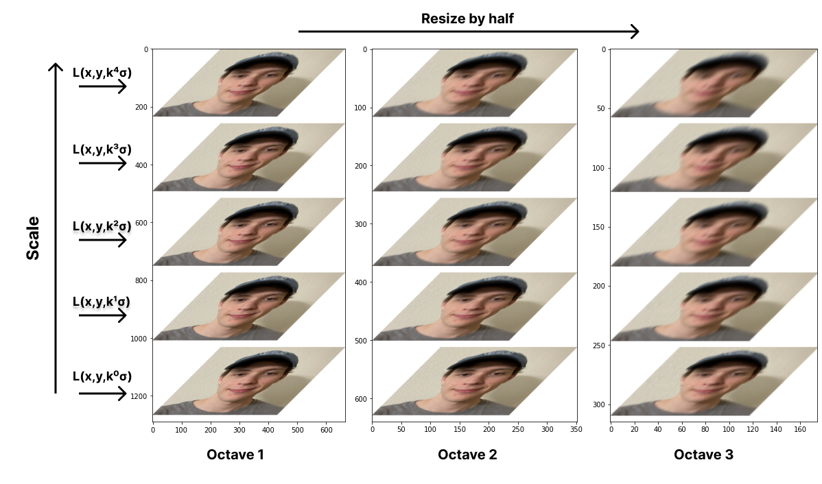
Difference of Gaussian
The motivation behind Difference of Gaussian DoG is to serve as a speedy alternative for blob detection while also maintaining scale invariance. Typically, a scale-normalized Laplacian of Gaussian (LoG) is used for this, but with a bit of clever math, DoG can acheive a good approximation of scale-normalized LoG efficiently as the smoothed image \(L\) can be used for scale-space feature description by image subtraction.
Proving DoG \(\approx\) LoG
The Laplacian of Gaussian for image \(I\) is given as:
\[\nabla^{2}L=\nabla^{2}(G\ast I)=\underbrace{\nabla^{2}G}_\textrm{LoG}\ast I\]LoG can be expanded to:
\[\frac{\partial^{2}G}{\partial x^{2}}=\frac{G(x,y,\sigma)}{\sigma^{2}} \left(\frac{x^2}{\sigma^2} - 1\right) \quad \frac{\partial^{2}G}{\partial y^{2}}=\frac{G(x,y,\sigma)}{\sigma^{2}} \left(\frac{y^2}{\sigma^2} - 1\right)\] \[\nabla^{2}G=\frac{\partial^{2}G}{\partial x^{2}} + \frac{\partial^{2}G}{\partial y^{2}} = \frac{G(x,y,\sigma)}{\sigma^{2}}\left(\frac{x^2 + y^2}{\sigma^2} - 2\right)\]Then the derivative of the Gaussian kernel can be expressed as:
\[\begin{align*} \frac{\partial G}{\partial \sigma} &= \sigma \left[ \frac{G(x,y,\sigma)}{\sigma^{2}} \left(\frac{x^2 + y^2}{\sigma^2} - 2\right) \right] = \sigma \nabla^{2}G \end{align*}\]Scale-normalized LoG is obtained by eliminating the \(\sigma^{-2}\) term:
\[\sigma^{2} \left[ \nabla^{2}G = \frac{G(x,y,\sigma)}{\sigma^{2}}\left(\frac{x^2 + y^2}{\sigma^2} - 2\right) \right] \Rightarrow \underbrace{\sigma^{2}\nabla^{2}G}_\textrm{Scale Norm LoG} = G(x,y,\sigma)\left(\frac{x^2 + y^2}{\sigma^2} - 2\right)\]Using this, we can take the finite difference approximation using nearby scales \(\sigma\) and \(k\sigma\) to discover the relationship between scale-normalized LoG and DoG.
\[\begin{align*} \frac{\partial G}{\partial \sigma} =\sigma \nabla^{2}G \approx \frac{G(x,y,k\sigma) - G(x,y,\sigma)}{k\sigma - \sigma} \\ \sigma \nabla^{2}G \approx \frac{G(x,y,k\sigma) - G(x,y,\sigma)}{\sigma(k - 1)} \\ \end{align*} \\\] \[\begin{align} (k-1)\underbrace{\sigma^{2}\nabla^{2}G}_\textrm{Scale Norm LoG} \approx \underbrace{G(x,y,k\sigma) - G(x,y,\sigma)}_\textrm{DoG} \end{align}\]This shows that taking the difference between two Gaussians with scales differing by constant factor \(k\), the \(\sigma^{2}\) term required for scale-normalized LoG is automatically incorperated. Factor (k - 1) remains constant for every \(\sigma\) which means that it will not influence extrema locality which is important for the following steps.
def gen_DoGs(octave): # Convert to grayscale before taking the difference

    for i, scale in enumerate(octave):
        octave[i] = cv.cvtColor(scale, cv.COLOR_BGR2GRAY)

    DoGs = []
    for i in range(len(octave ) - 1):
        sub_img = octave[i + 1] - octave[i] # Equation (3)
        DoGs.append(sub_img)

    return DoGs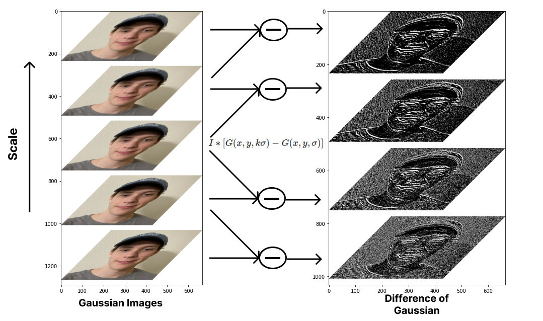
Local Extrema Detection
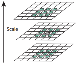
Now that we have a good representation of regions with rapid changes in the image from DoG, we can locate the extrema and use them as a representation of keypoints in the image. For detecting extrema, points are sampled in the image and then compared to its eight neighbors in the current scale and nine neighbors in the previous scale and next scale. It is selected as a keypoint candidate if the value is greater than or less than all of its neighbors.
def extrema_detection(DoGs, s_idx): # Using neighboring scales

    s_prev, s_curr, s_next = DoGs[s_idx - 1:s_idx + 2]
    candidate_map = np.full_like(s_curr, fill_value=0)
    pad = 1
    # Reference for neighboring points
    neighs = [
        (i,j) for i in range(-pad, pad + 1)
            for j in range(-pad, pad + 1) if i or j
    ]
    candidates = []

    for i in range(pad, s_curr.shape[0] - pad):
        for j in range(pad, s_curr.shape[1] - pad):
            sample = s_curr[i, j]
            for neigh in neighs:
                ni, nj = neigh[0] + i, neigh[1] + j
                maxima = sample > s_curr[ni, nj] \
                    and sample > s_prev[ni, nj] and sample > s_next[ni, nj]
                minima = sample < s_curr[ni, nj] \
                    and sample < s_prev[ni, nj] and sample < s_next[ni, nj]
                if not maxima and not minima:
                    break
            if maxima or minima:
                candidate_map[i, j] = sample
                candidates.append((j, i, s_idx))

    return candidate_map, candidates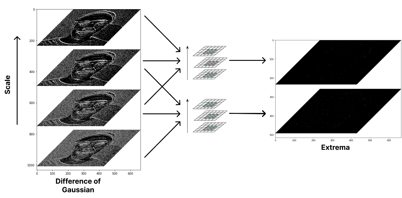
Keypoint Localization and Refinement
Naturally, the keypoints extracted from the previous step are crudely localized because of the quantization used in constructing the scale-space. As a result, there can be many unreliable keypoint candidates because their locations are approximations of the extrema. SIFT refines the keypoint candidates by fitting their local neighborhoods with the second order Taylor expansion of the DoG function. Then it interpolates the discrete approximations from the previous step to give a better representation of the extrema.
Interpolation of Nearby Data
This is done by using the second order Taylor expansion for the DoG function with a sample keypoint \(\mathbf z_i = [x_i \ y_i \ \sigma_i]^{T}\) and shifting it by an offset \(\mathbf z = [x \ y \ \sigma]^{T}\) so that the origin is at the sample’s location.
\[D(x,y,\sigma) = D(\mathbf{z_i}+\mathbf z) \approx D(\mathbf{z_i}) + \bigg(\frac{ \partial D}{\partial \mathbf z}\bigg)^T\bigg|_{\mathbf z=\mathbf z_i}\mathbf z + \frac 1 2 \mathbf z^T\frac{ \partial^2 D}{\partial \mathbf z^2}\bigg|_{\mathbf z=\mathbf z_i} \mathbf z\]To locate an extremum \(\mathbf{\hat z}\), take the derivative of the Taylor expansion with respect to \(\mathbf{z}\) and set it to 0:
\[\begin{align*} \frac{\partial}{\partial \mathbf{z}} \bigg[D(\mathbf{z_i}) + \bigg(\frac{ \partial D}{\partial \mathbf z}\bigg)^T\mathbf z + \frac 1 2 \mathbf z^T\frac{ \partial^2 D}{\partial \mathbf z^2} \mathbf z \bigg] = \frac{ \partial D}{\partial \mathbf z} + \frac{ \partial^2 D}{\partial \mathbf z^2} \mathbf z \\ \end{align*}\]Set it equal to 0 and solve for extremum \(\mathbf{\hat z}\):
\[\begin{align} \frac{ \partial D}{ \partial \mathbf z} + \frac{ \partial^2 D}{\partial \mathbf z^2} \mathbf{\hat z} = 0 \quad \Rightarrow \frac{ \partial^2 D}{\partial \mathbf z^2} \mathbf{\hat z} = -\frac{ \partial D}{ \partial \mathbf z} \quad \Rightarrow \mathbf{\hat z} = -\frac{ \partial^2 D}{\partial \mathbf z^2}^{-1}\frac{ \partial D}{ \partial \mathbf z} \end{align}\]def second_order_TE_inter(neigh):
# Compute first deriv (Gradient) in Taylor series
# on sample kp with adjacent pixels
dx = (neigh[1, 1, 2] - neigh[1, 1, 0]) / 2
dy = (neigh[1, 2, 1] - neigh[1, 0, 1]) / 2
ds = (neigh[2, 1, 1] - neigh[0, 1, 1]) / 2
grad = np.array([dx, dy, ds])
# Compute second deriv (Hessian) in Taylor series on sample kp with
# adjacent pixels
candidate = neigh[1, 1, 1]
dxx = neigh[1, 1, 2] - 2 * candidate + neigh[1, 1, 0]
dyy = neigh[1, 2, 1] - 2 * candidate + neigh[1, 0, 1]
dss = neigh[2, 1, 1] - 2 * candidate + neigh[0, 1, 1]
dxy = (neigh[1, 2, 2] - neigh[1, 2, 0] - \
neigh[1, 0, 2] + neigh[1, 0, 0]) / 4
dxs = (neigh[2, 1, 2] - neigh[2, 1, 0] - \
neigh[0, 1, 2] + neigh[0, 1, 0]) / 4
dys = (neigh[2, 2, 1] - neigh[2, 0, 1] - \
neigh[0, 2, 1] + neigh[0, 0, 1]) / 4
hess = np.array([
[dxx, dxy, dxs],
[dxy, dyy, dys],
[dxs, dys, dss]
])
# Avoid inverting singular matrix
if np.linalg.det(hess) == 0:
return np.zeros(shape=3), 0
# Solve for extremum and get the contrast at that point
z_hat = -np.linalg.inv(hess).dot(grad) # Equation (4)
contrast = candidate + grad.T.dot(z_hat) / 2 # Equation (5)
return z_hat, contrastEliminating low contrast points
If \(\mathbf{\hat z}\) is greater than 0.5 or less than -0.5 for any dimension, then that indicates that the extremum lies outside the neighborhood of the sample so the candidate keypoint is discarded. Otherwise, add the offset \(\mathbf{\hat z}\) to the candidate keypoint \(\mathbf{z_i}\) to get the updated extremum \(\mathbf{z_i} + \mathbf{\hat z}\). This process is done iteratively until the offset is valid. If its not valid by the final iteration, then it is discarded. We can substitute \(\mathbf z\) in the Taylor expansion with \(\mathbf{\hat{z}}\) to get the interpolated value at the localized extremum:
\[\begin{align*} D(\mathbf{z_i}+\mathbf{\hat z}) = D(\mathbf{z_i}) + \bigg(\frac{ \partial D}{\partial \mathbf z}\bigg)^T\bigg|_{\mathbf z=\mathbf z_i} \mathbf{\hat z} + \frac 1 2 \mathbf{\hat z}^T\frac{ \partial^2 D}{\partial \mathbf z^2}\bigg|_{\mathbf z=\mathbf z_i} \mathbf{\hat z} \end{align*}\] \[\begin{align} = D(\mathbf{z_i}) + \frac 1 2 \bigg(\frac{ \partial D}{\partial \mathbf z}\bigg)^T\bigg|_{\mathbf z=\mathbf z_i} \mathbf{\hat z} \end{align}\]The value represents the contrast at that point. If |\(D(\mathbf{z_i}+\mathbf{\hat z})\)|\(< 0.03\), it is consider to be low contrast and discarded.
def keypoint_inter(DoGs, cands, max_it=5, con_thresh=0.03):

    refined = []
    for cand in cands:
        (x, y, s) = cand
        in_neigh, outside = False, False

        for i in range(max_it):
            s_prev, s_curr, s_next = DoGs[s - 1:s + 2]
            neighborhood = np.stack([
                s_prev[y - 1:y + 2, x - 1:x + 2],
                s_curr[y - 1:y + 2, x - 1:x + 2],
                s_next[y - 1:y + 2, x - 1:x + 2],
            ]).astype(np.float32) / 255

            # calculate extremum in the second order Taylor expansion
            offset, contrast = second_order_TE_inter(neighborhood)

            in_neigh = abs(offset[0]) < 0.5
            in_neigh &= abs(offset[1]) < 0.5
            in_neigh &= abs(offset[2]) < 0.5

            # stop if the extremum is in the neighborhood
            if in_neigh: break

            # update extremum
            x += int(round(offset[0]))
            y += int(round(offset[1]))
            s += int(round(offset[2]))

            outside = (x < 1 or x >= s_curr.shape[1] - 1)
            outside |= (y < 1 or y >= s_curr.shape[0] - 1)
            outside |= (s < 1 or s >= len(DoGs) - 1)

            # discard if extremum is outside the image or scale-space
            if outside: break

        if not in_neigh or outside or abs(contrast) < con_thresh:
            continue
        else:
            x += int(round(offset[0]))
            y += int(round(offset[1]))
            s += int(round(offset[2]))
            refined.append((x, y, s, abs(contrast)))

    refined_map = np.full_like(DoGs[0], fill_value=0)
    for p in refined:
        refined_map[p[1], p[0]] = p[3] * 255
    return refined_map, refined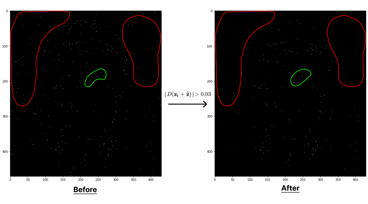
The red region shows some extrema that were discarded due to having low contrast. The green region shows extrema that shifted by the offset from the interpolation.
Eliminating edge responses
As you may have noticed in the DoG images, the contours on my face and hat were easily discernible which means that it had a strong response along these edges and curves. Some of the points along the edges are coarsely located and easily influenced to small amounts of noise resulting in undesirable extrema. This process will also eliminate other erroneous extremas with no structure.
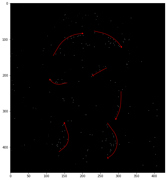
Using the 2D Hessian \(\mathbf H\) of the DoG, information about the local structure around a keypoint can be obtained. The eigenvalues of \(\mathbf H\) can provide the maximal and minimal principle curvatures at a DoG point. Edges will have a large principal curvature orthogonal to the contour and a small one along the contour.
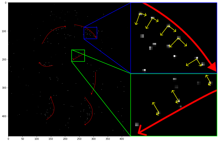
All of the keypoints in the green region should be discarded. In the blue, the points along the ridge should be kept because the orthogonal principal curvature is nearly the same as the one along the contour, indicating that it is not on an edge.
SIFT will discard the keypoints whose eigenvalue ratio is more than threshold \(r\), as this indicates that the point lies on an edge. \(r\) is related to the ratio of the Hessian determinant and its trace.
\[\mathbf{H} = \begin{bmatrix} D_{xx} & D_{xy} \\ D_{xy} & D_{yy} \end{bmatrix} \quad \quad \frac {\text{Tr}(\mathbf{H})^2} {\text{Det}(\mathbf{H})} = \frac {(\lambda_{1} + \lambda_{2})^2}{\lambda_{1}\lambda_{2}} < \frac{(r+1)^2}{r}\]This relationship can also be expressed as:
\[\begin{align} \frac {\text{Tr}(\mathbf{H})^2} {\text{Det}(\mathbf{H})} < \frac{(r+1)^2}{r} \quad \Rightarrow \quad r\text{Tr}(\mathbf{H})^2 < (r+1)^2\text{Det}(\mathbf{H}) \end{align}\]def elim_edge_responses(DoGs, cands, r=10):
refined = []
for cand in cands:
(x, y, s, _) = cand
neigh = DoGs[s][y - 1:y + 2, x - 1:x + 2].astype(np.float32) / 255
dxx = neigh[1, 2] - 2 * neigh[1, 1] + neigh[1, 0]
dyy = neigh[2, 1] - 2 * neigh[1, 1] + neigh[0, 1]
dxy = (neigh[2, 2] - neigh[2, 0] - neigh[0, 2] + neigh[0, 0]) / 4
H = np.array([
[dxx, dxy],
[dxy, dyy]
])
tr_H, det_H = np.trace(H), np.linalg.det(H)
lhs = r * (tr_H ** 2) # Lefthand side of condition (6)
rhs = ((r + 1) ** 2) * det_H # Righhand side of condition (6)
if lhs < rhs:
refined.append(cand)
refined_map = np.full_like(DoGs[0], fill_value=0)
for p in refined:
refined_map[p[1], p[0]] = p[3] * 255
return refined_map, refined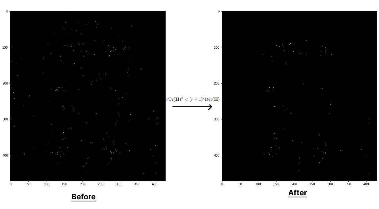
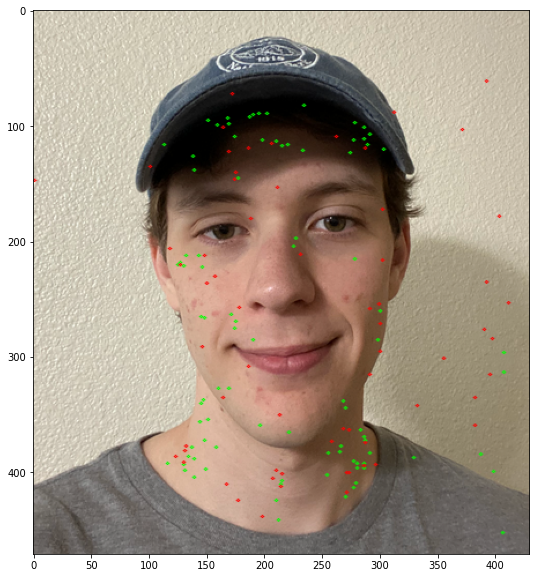
The green dots are showing the keypoints from the second scale and red dots are from the thrid scale after refinement.
Descriptor Orientation
The descriptors are structured around a set of weighted histograms of the gradient orientation taken at the neighboring regions of the keypoint. The most dominant gradient orientation over a keypoint neighborhood is provided by the strongest gradient angle in the region and is selected as the reference orientation, allowing for rotation invariance for the resulting descriptor. The size of the region depends on the scale and octave that the keypoint was located in.
For each keypoint, the gradient magnitude \(m\) and the gradient angle \(\theta\) are computed:
\[L(x,y,\sigma) = G(x,y,\sigma) \ast I(x,y) \\\] \[\begin{align} m(x,y) = \sqrt{(L(x+1,y)-L(x-1,y))^2 + (L(x,y+1)-L(x,y-1))^2} \\ \end{align}\] \[\begin{align} \theta(x,y) = \arctan\left(\frac{ L(x,y+1)-L(x,y-1)}{L(x+1,y)-L(x-1,y)}\right) \end{align}\]
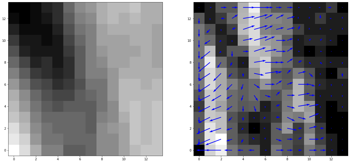
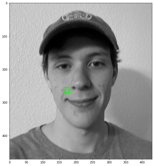
The left image shows the patch of a sample keypoint from the green region below. The right image shows the gradient magnitudes represented by the color with their respective gradient angles.
SIFT accumulates the local distribution of the gradient angle within a region using a histogram composed of 36 bins for every 10 degrees in a full rotation (360 degrees). The amount added to a bin depends on the product of the gradient magnitude and the contribution weight at that particular point. \(\lambda_{ori}\) is used to adjust the reach of the distribution.
\[\begin{align} \text{Contribution weight at (x,y):} \quad c_{x,y}^{ori} = \exp\left(\frac{-(x^2 + y^2)}{2(\lambda_{ori}\sigma)^2}\right) \\ \end{align}\] \[\begin{align} \text{Bin index at (x,y):} \quad b_{x,y}^{ori} = \frac{\theta_{x,y} n_{bins}}{360} \end{align}\]N_BINS = 36 # number of bins in gradient histogram
LAMBDA_ORI = 1.5 # scale the reach of the gradient distribution
R = 3 # Radius of the gaussian window
T = 0.80 # threshold for considering local maxima in the histogram
def gen_hist(kp, scale, octave, o_idx):
hist = np.zeros(N_BINS)
gauss_img = octave[int(kp.size)] / 255
shape = gauss_img.shape
rad = int(round(R * scale))
for y_shift in range(-rad, rad + 1):
y_r = int(round(kp.pt[1]) / float(2 ** o_idx)) + y_shift
if y_r < 1 or y_r >= shape[0] - 2:
continue
for x_shift in range(-rad, rad + 1):
x_r = int(round(kp.pt[0]) / float(2 ** o_idx)) + x_shift
if x_r < 1 or x_r >= shape[1] - 1:
continue
# compute gradient magnitudes and
# orientation from the current patch
dx = gauss_img[y_r, x_r + 1] - gauss_img[y_r, x_r - 1]
dy = gauss_img[y_r + 1, x_r] - gauss_img[y_r - 1, x_r]
mag = math.sqrt(dx ** 2 + dy ** 2) # Equation (7)
ori = np.rad2deg(np.arctan2(dy, dx)) # Equation (8)
# compute sample contribution weight and bin index, then
# place in hist
# Equation (9)
con = np.exp(-(x_shift ** 2 + y_shift ** 2) / (2 * scale ** 2))
# Equation (10)
bin_idx = int(round(ori * N_BINS / 360.))
hist[bin_idx % N_BINS] += con * mag
return histSmoothing the histogram by weighting nearby bins and averaging them.
def smooth_hist(hist):

    smooth = []

    # Smoothing histogram by weighting nearby bins and averaging them
    for i in range(N_BINS):
        smooth_mag = 6 * hist[i] + 4 * (hist[i - 1] + hist[(i + 1) % N_BINS])
        smooth_mag += hist[i - 2] + hist[(i + 2) % N_BINS]
        smooth_mag /= 16.
        smooth.append(smooth_mag)

    return smooth
After computing the smoothed histogram, the orientation with the greatest magnitude (peak) is selected as its reference orientation. Additionally, if any other orientation contains a magnitude that is greater than 80% of the peak, then a new keypoint gets created with the same location and is assigned that orientation instead.
def compute_reference(kp, smooth):

    max_ori = max(smooth)

    # sample window
    band = (smooth > np.roll(smooth, 1), smooth > np.roll(smooth, -1))
    peaks = np.where(band[0] & band[1])[0]

    ori_kps = []
    # Extract the reference orientations
    for p_idx in peaks:
        p_val = smooth[p_idx]
        if p_val < T * max_ori:
            continue
        l_val = smooth[(p_idx - 1) % N_BINS]
        r_val = smooth[(p_idx + 1) % N_BINS]

        # compute the reference index
        norm_p_idx = p_idx + 0.5 * (l_val - r_val)
        norm_p_idx /= l_val - 2 * p_val + r_val
        norm_p_idx %= N_BINS

        # compute the reference orientation
        ori = 360. - norm_p_idx * 360. / N_BINS
        ori_kp = cv.KeyPoint(*kp.pt, kp.size, ori, kp.response, kp.octave)
        ori_kps.append(ori_kp)

    return ori_kps
All together
def compute_orientations(keypoints, octaves, o_idx, k):

    octave = octaves[o_idx]
    kps, hists = [], []

    for kp in keypoints:
        scale = LAMBDA_ORI * kp.size / (2 ** o_idx)

        hist = gen_hist(kp, scale, octave, o_idx)
        smooth = smooth_hist(hist)
        ori_kps = compute_reference(kp, smooth)

        kps += ori_kps
        hists.append((hist, smooth))

    return hists, kps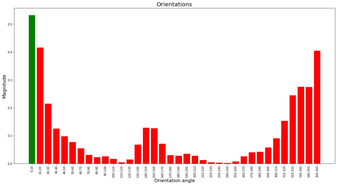
The green bar shows the orientation that was selected for the feature descriptor and the red bars are the orientations that didn’t pass the threshold.
Descriptor Construction
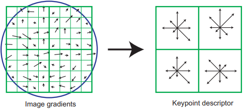
A descriptor is constructed for the keypoint by partitioning the normalized patch into a set of \(n_{hists} \times n_{hists}\) (where \(n_{hists}=4\)) weighted histograms to form a spatial grid of the gradient orientations from different regions of the normalized patch. Instead of using 36 spatial bins like the previous step, 8 are used for binning the angles (\(n_{ori}=8\)).
N_HISTS = 4
N_ORI = 8
LAMBDA_DESC = 3
SATURATE = 0.2

def accum_hists(kp, octaves, oct_idx, scale_idx): # sample varibales

    gauss_img = octaves[oct_idx][scale_idx] / 255
    num_rows, num_cols = gauss_img.shape
    pt = np.round(kp.size * np.array(kp.pt)).astype(int)
    deg = N*HISTS / 360.
    cos_angle = np.cos(np.deg2rad(kp.angle))
    sin_angle = np.sin(np.deg2rad(kp.angle))
    weight = -0.5 / ((0.5 \* N_HISTS) \*\* 2)

    # compute the region boundary for the histogram of the normalized patch
    hist_size = LAMBDA_DESC * 0.5 * kp.size
    r = int(round(hist_size * np.sqrt(2) * (N_HISTS + 1) * 0.5))
    r = int(min(r, np.sqrt(num_rows ** 2 + num_cols ** 2)))

    # accumulate samples of normalized patch for the bins
    accum = []
    for y in range(-r, r + 1):
        for x in range(-r, r + 1):
            # compute normalized coordinates
            y_ori = x * sin_angle + y * cos_angle
            x_ori = x * cos_angle - y * sin_angle
            y_bin = (y_ori / hist_size) + 0.5 * N_HISTS - 0.5
            x_bin = (x_ori / hist_size) + 0.5 * N_HISTS - 0.5

            # verify if sample belongs in a bin
            valid_bin = y_bin > -1 and y_bin < N_HISTS
            valid_bin &= x_bin > -1 and x_bin < N_HISTS
            if not valid_bin:
                continue

            # verify if sample is in the patch
            r_patch = int(round(pt[1] + y))
            c_patch = int(round(pt[0] + x))
            in_patch = r_patch > 0 and r_patch < num_rows - 1
            in_patch &= c_patch > 0 and c_patch < num_cols - 1
            if not in_patch:
                continue

            # compute normalized gradient orientation
            dx = gauss_img[r_patch, c_patch + 1] \
                - gauss_img[r_patch, c_patch - 1]
            dy = gauss_img[r_patch - 1, c_patch] \
                - gauss_img[r_patch + 1, c_patch]
            grad_mag = np.sqrt(dx ** 2 + dy ** 2)
            grad_ori = np.rad2deg(np.arctan2(dy, dx)) % 360

            # compute contribution of the sample
            con = np.exp(
                weight * (
                    (y_ori / hist_size) ** 2 + (x_ori / hist_size) ** 2
                )
            )
            mag = con * grad_mag
            ori = (grad_ori - kp.angle) * deg

            accum.append((y_bin, x_bin, mag, ori))
    return accum
Trilinear interpolation is used to spread the weight across neighboring spatial bins and across neighboring angle bins instead of having it concentrated in a single bin. This creates more robust descriptors when trying to match them with images taken from different perspectives.
def trilinear_inter(accum):

    hist = np.zeros((N_HISTS + 2, N_HISTS + 2, N_ORI))
    for (r_bin, c_bin, mag, o_bin) in accum:
        r_idx, c_idx, o_idx = np.floor([r_bin, c_bin, o_bin]).astype(int)
        row_diff, col_diff, ori_diff = \
            r_bin - r_idx, c_bin - c_idx, o_bin - o_idx

        if o_idx < 0:
            o_idx += N_ORI
        if o_idx >= N_ORI:
            o_idx -= N_ORI

        # update the eight values
        pt1 = mag * row_diff * col_diff * ori_diff
        pt2 = mag * row_diff * col_diff * (1 - ori_diff)
        pt3 = mag * row_diff * (1 - col_diff) * ori_diff
        pt4 = mag * row_diff * (1 - col_diff) * (1 - ori_diff)
        pt5 = mag * (1 - row_diff) * col_diff * ori_diff
        pt6 = mag * (1 - row_diff) * col_diff * (1 - ori_diff)
        pt7 = mag * (1 - row_diff) * (1 - col_diff) * ori_diff
        pt8 = mag * (1 - row_diff) * (1 - col_diff) * (1 - ori_diff)

        hist[r_idx + 1, c_idx + 1, o_idx] += pt8
        hist[r_idx + 1, c_idx + 1, (o_idx + 1) % N_ORI] += pt7
        hist[r_idx + 1, c_idx + 2, o_idx] += pt6
        hist[r_idx + 1, c_idx + 2, (o_idx + 1) % N_ORI] += pt5
        hist[r_idx + 2, c_idx + 1, o_idx] += pt4
        hist[r_idx + 2, c_idx + 1, (o_idx + 1) % N_ORI] += pt3
        hist[r_idx + 2, c_idx + 2, o_idx] += pt2
        hist[r_idx + 2, c_idx + 2, (o_idx + 1) % N_ORI] += pt1
    return hist
The accumulated array of histograms after interpolation is encoded into a feature vector \(\mathbf{f}\) of length \(n_{hists} \times n_{hists} \times n_{ori} = 128\). The vector is normalized and then saturated by 20% of the maximum value. This seeks to reduce the impact of non-linear illumination changes. Finally, the vector is renormalized by the product of 512 and quantized to 8 bit integers. This aims to accelerate the computation of distances between feature vectors when matching.
def gen_descriptors(keypoints, octaves, oct_idx, scale_idx):

    descriptors = []
    samples = []

    for kp in keypoints:
        # accumlate the histograms
        accum = accum_hists(kp, octaves, oct_idx, scale_idx)

        # apply trilinear interpolation
        hist = trilinear_inter(accum)

        # build the feature vector
        sample_hist = hist[1:-1, 1:-1, :]
        f = sample_hist.flatten()
        # normalize and saturate feature vector
        threshold = np.linalg.norm(f) * SATURATE
        f[f > threshold] = threshold
        f /= max(np.linalg.norm(f), 1e-7)

        # renormalize and quantize into 8 bit integer
        f = np.round(512 * f)
        f[f < 0], f[f > 255] = 0, 255
        descriptors.append(f)

    for sample in descriptors:
        samples.append(sample.reshape(4, 4, 8))

    return np.array(descriptors, dtype=np.uint8), samples
What’s next?
Next, I’ll be explaining how to match the feature keypoints gathered from using SIFT in order to stitch images together.
Additional Notes
The code I provided is a barebones implementation I had done, so it is likely suboptimal and prone to errors. I found that the original paper was insufficient in terms of providing information on how to construct the algorithm.
I did a little digging and found an article that goes into rigorous detail on how to go about implementing the algorithm. I referenced it a lot when constructing the algorithm but left out some details. If I didn’t explain something very well or you would like to understand the algorithm more clearly, I suggest you take a look at it.